Link: https://juliaactuary.org/tutorials/yield-curve-fitting/
Graphic:
Excerpt:
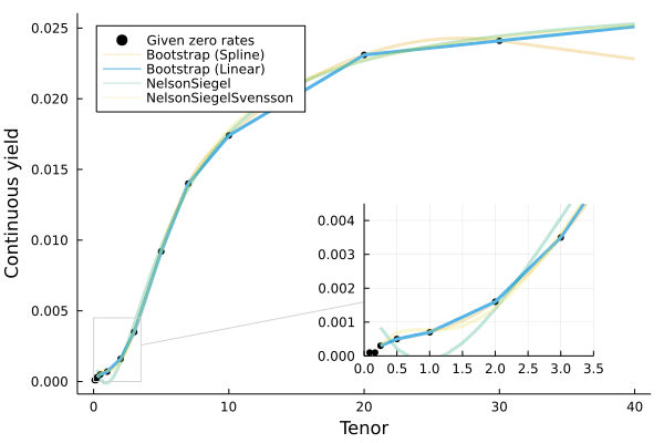
Given rates and maturities, we can fit the yield curves with different techniques in Yields.jl.
Below, we specify that the rates should be interpreted as Continuously compounded zero rates:
using Yields

rates = Continuous.([0.01, 0.01, 0.03, 0.05, 0.07, 0.16, 0.35, 0.92, 1.40, 1.74, 2.31, 2.41] ./ 100)
mats = [1/12, 2/12, 3/12, 6/12, 1, 2, 3, 5, 7, 10, 20, 30]
Then fit the rates under four methods:
- Nelson-Siegel
- Nelson-Siegel-Svennson
- Boostrapping with splines (the default
Bootstrapoption) - Bootstrapping with linear splines
ns =  Yields.Zero(NelsonSiegel(),                   rates,mats)
nss = Yields.Zero(NelsonSiegelSvensson(),           rates,mats)
b =   Yields.Zero(Bootstrap(),                      rates,mats)
bl =  Yields.Zero(Bootstrap(Yields.LinearSpline()), rates,mats)
That’s it! We’ve fit the rates using four different techniques. These can now be used in a variety of ways, such as calculating the present_value, duration, or convexity of different cashflows if you imported ActuaryUtilities.jl
Publication Date: 19 Jun 2022, accessed 22 Jun 2022
Publication Site: JuliaActuary